Introduction
Picture this: you've just received a letter from your pension administrator offering two options — a $600,000 lump sum today, or $50,000 per year for the next 25 years. Which is worth more?
Most people guess wrong. Without running the actual math, the lump sum feels safer, more concrete. But the ordinary annuity formula exists precisely to answer this question — and the answer isn't always what you'd expect.
This article is written for retirees, federal employees weighing FERS or CSRS pension elections, and anyone trying to make sense of recurring payment streams.
Most explanations of annuity math either skip the formulas entirely or bury you in equations without context. This guide covers the formulas and the worked arithmetic — with enough real-world framing to make the numbers useful for actual decisions.
Key Takeaways
- An ordinary annuity = equal payments made at the end of each period (mortgages, pension disbursements)
- The present value (PV) formula tells you what a future payment stream is worth in today's dollars
- Future value (FV) shows how much recurring contributions will accumulate over time
- Annuity due pays at the beginning of each period, making it worth more than an ordinary annuity by a factor of (1 + r)
- Three inputs drive every calculation: payment amount, interest/discount rate, and number of periods
What Is an Ordinary Annuity?
An ordinary annuity is a fixed series of equal payments made at the end of each compounding period over a defined time horizon. Every payment is identical in amount, and every payment lands at period-end — not before.
This structure matters because of the time value of money — the principle that a dollar received today is worth more than a dollar received a year from now, because today's dollar can be invested and grow. Ordinary annuities let you apply this principle systematically to a stream of future cash flows.
Two closely related concepts are worth distinguishing:
- Annuity due — identical structure, except payments arrive at the beginning of each period rather than the end. Rent is a classic example; landlords typically collect upfront.
- Perpetuity — a payment stream with no end date, continuing indefinitely. No fixed term, no formula for n.
Real-world ordinary annuity examples include monthly mortgage payments, car loan installments, and OPM retirement annuity disbursements, which OPM pays on the first business day of the following month — covering the previous month, consistent with end-of-period timing.
Present Value of an Ordinary Annuity: Formula and Calculation
Present value answers a specific question: how much money do you need today, invested at a given rate, to fund every future payment in the annuity? This is the number that makes lump-sum-vs.-payment-stream comparisons possible.
The PV Formula
Per OpenStax Principles of Finance, the formula is:
PV = PMT × [1 − (1 + r)^(−n)] / r
Where:
- PMT = the periodic payment amount (fixed and equal each period)
- r = the discount rate per period (not the annuity's stated interest rate — more on this below)
- n = total number of payment periods
Understanding the Discount Rate
The discount rate is not the interest rate printed on the annuity contract. It represents the return you could realistically earn on an alternative investment of comparable risk — your opportunity cost.
If you could invest safely in a comparable bond yielding 6%, then 6% is the appropriate discount rate. A lower rate inflates the annuity's apparent value; a higher rate cuts it. The GAO documented this effect precisely: a pension benefit valued at $62,643 using a 3.65% Treasury rate dropped to $32,453 when a 6.02% corporate bond rate was applied instead — same benefit, very different present values.
Worked Example: PV Calculation
Inputs: PMT = $50,000 | r = 6% (0.06) | n = 25 years
Step 1: Calculate (1.06)^(−25) = 1 / (1.06)^25 = 1 / 4.2919 ≈ 0.2330
Step 2: Subtract from 1: 1 − 0.2330 = 0.7670
Step 3: Divide by r: 0.7670 / 0.06 = 12.7833
Step 4: Multiply by PMT: $50,000 × 12.7833 = $639,167.81
Apply this to a real decision: a $600,000 lump sum offer versus a $50,000/year stream for 25 years. Discounted at 6%, the payment stream is worth $639,167.81 — the annuity wins by roughly $39,000 on a present-value basis.
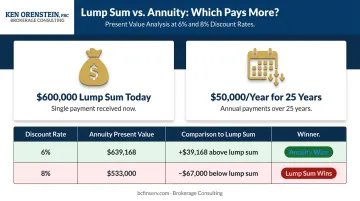
Change the discount rate to 8%, and the PV drops to around $533,000 — suddenly the lump sum looks better. Before accepting any lump-sum offer, confirm which discount rate is being used and whether it reflects realistic alternatives available to you.
FERS and CSRS retirees regularly face pension election decisions — lump-sum options, survivor benefit trade-offs — where present value comparisons are essential. Ken Orenstein at Brokerage Consulting works through this analysis for federal employees, applying the calculations to specific plan terms and individual tax situations. A no-cost consultation is available at bcfinserv.com/request-a-quote or by calling (888) 315-3608.
Future Value of an Ordinary Annuity: Formula and Calculation
PV tells you what future payments are worth today. FV answers the saver's question: what will my recurring contributions be worth at the end of the term?
FV is the saver's formula. Use it when projecting how quarterly retirement deposits, annual TSP contributions, or any regular savings habit will compound over time.
The FV Formula
FV = PMT × [(1 + i)^n − 1] / i
Where i and n match the compounding interval (not necessarily annual).
How Compounding Works Inside the Formula
Each payment is deposited at the end of its period, then earns compound interest for the remaining periods. The first payment has the most time to grow — it compounds for nearly the entire term. The last payment earns nothing, deposited at the final period with no time remaining.
This staggered compounding is what the formula captures mathematically. The bracket term [(1 + i)^n − 1] / i sums all those individual growth amounts into a single factor.
Worked Example: FV Calculation
Inputs: PMT = $1,000/quarter | Annual rate = 6.5% | Term = 15 years
Step 1 — Derive periodic rate: i = 6.5% ÷ 4 = 1.625% (0.01625) per quarter
Step 2 — Set n: 15 years × 4 quarters = 60 periods
Step 3 — Apply formula: FV = $1,000 × [(1.01625)^60 − 1] / 0.01625
(1.01625)^60 ≈ 2.6310
FV = $1,000 × [2.6310 − 1] / 0.01625 = $1,000 × 1.6310 / 0.01625 = $1,000 × 100.34 = $100,336.68
Solving for the Required Payment (PMT)
The FV formula rearranges to solve for PMT when you have a savings target in mind:
PMT = FV × i / [(1 + i)^n − 1]
Example: want $10,000 in 8 years with 5% annual compounding?
PMT = $10,000 × 0.05 / [(1.05)^8 − 1] = $500 / 0.4775 ≈ $1,047.22/year
Use this rearrangement for sinking fund planning. It answers a precise question: given a target balance and a deadline, what do I need to save each period?
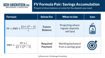
| Formula | Solves For | When to Use |
|---|---|---|
| FV = PMT × [(1 + i)^n − 1] / i | Future balance | Projecting where regular deposits will land |
| PMT = FV × i / [(1 + i)^n − 1] | Required payment | Working backward from a savings goal |
Ordinary Annuity vs. Annuity Due: Understanding the Difference
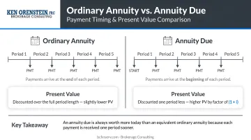
The distinction is simple: ordinary annuity payments come at period-end, annuity due payments come at period-start.
| Structure | Payment Timing | Real-World Examples |
|---|---|---|
| Ordinary annuity | End of each period | Pension disbursements, SPIA payouts, structured settlements |
| Annuity due | Beginning of each period | Rent, insurance premiums, prepaid lease payments |
Why Timing Changes the Math
Because annuity due payments arrive one period earlier, each payment has one additional compounding period to grow (for FV) or one less discounting period (for PV). The result: annuity due is always worth more than an otherwise identical ordinary annuity.
The Formula Adjustment
Translating that timing advantage into math is straightforward. Both PV and FV for an annuity due are derived by multiplying the ordinary annuity result by (1 + r):
- PV (annuity due) = PV (ordinary) × (1 + r)
- FV (annuity due) = FV (ordinary) × (1 + r)
That single multiplier captures the full timing difference.
Side-by-Side Dollar Comparison
Using the same inputs from the PV example ($50,000/year, 25 years, 6%):
| Structure | Present Value |
|---|---|
| Ordinary annuity | $639,167.81 |
| Annuity due | $677,517.88 |
| Timing difference | $38,350.07 |
Nearly $38,400 in present-value terms — just from receiving payments at month-start versus month-end. For retirees comparing pension options or SPIA structures, this gap is material — and worth clarifying with your advisor before signing any contract.
Key Factors That Affect the Ordinary Annuity Formula
Three inputs control every outcome. Understanding how each one behaves helps you build more accurate projections:
- Payment amount (PMT): Directly proportional — double the payment, double the PV and FV. No compounding effect on the payment itself — it scales linearly.
- Discount/interest rate (r): The most sensitive input. A higher rate reduces PV (future cash is worth less today) but increases FV — and even small rate shifts produce large dollar differences.
- Number of periods (n): More periods grow FV substantially through compounding, but add diminishing value to PV — payments 30 years out are discounted so heavily they contribute little to the present total.
Those three variables drive the math. Two external forces, however, can quietly undermine what the numbers actually mean in the real world:
Two external factors that skew real-world results:
- Inflation: The FV formula produces a nominal result. Federal Reserve Education notes that inflation reduces purchasing power for those with fixed income — meaning $100,000 accumulated in 20 years may buy far less than $100,000 today. Never confuse nominal FV with real purchasing power.
- Compounding frequency: Monthly compounding requires a monthly rate (annual rate ÷ 12) and monthly n (years × 12). Mismatching these is among the most common calculation errors. Always align i and n to the same interval.
Common Misconceptions About Ordinary Annuity Calculations
Confusing Discount Rate with the Annuity's Interest Rate
The discount rate is a valuation input — chosen by the analyst based on opportunity cost. The stated interest rate is a contractual feature of the annuity product. They are different numbers for different purposes. If you plug the annuity's stated rate into a PV analysis where your opportunity cost is higher, you'll overvalue the payment stream — and overpay for a lump-sum payout.
Assuming Higher FV Always Means a Better Deal
A larger future value reflects contributions plus interest — nothing more. It doesn't account for inflation eroding real purchasing power, taxes owed on distributions, or what the same contributions might have earned in a higher-return vehicle. FV is a starting point for analysis, not a conclusion.
Treating Ordinary Annuity and Annuity Due as Interchangeable
Many people apply the ordinary annuity formula without checking whether payments occur at period-start or period-end. As shown above, that error produces a result that's off by the factor (1 + r) — a $38,000 mistake on a $50,000/year stream at 6%. Always confirm payment timing in your contract before running any formula.
Frequently Asked Questions
What is the ordinary annuity formula?
There are two: PV = PMT × [1 − (1 + r)^(−n)] / r for present value, and FV = PMT × [(1 + i)^n − 1] / i for future value. PMT is the fixed periodic payment, r (or i) is the rate per period, and n is the total number of periods. Both formulas assume equal, end-of-period payments.
What is an ordinary annuity?
An ordinary annuity is a series of equal payments made at the end of each period over a fixed term. Common examples include monthly mortgage repayments, car loan installments, and annual pension disbursements where payments cover the prior month.
What is the formula for annuity due?
Annuity due payments are made at the beginning of each period. Both PV and FV are calculated by multiplying the ordinary annuity result by (1 + r): PV (due) = PV (ordinary) × (1 + r) and FV (due) = FV (ordinary) × (1 + r).
What are the two types of annuities called?
The two timing-based types are ordinary annuity (end-of-period payments) and annuity due (beginning-of-period payments). This single timing difference shifts every PV and FV result upward for annuity due, since each payment has one extra compounding period.
What is the accumulated value of an annuity paying $100/year for 10 years at 5% compounded annually?
Using FV = $100 × [(1.05)^10 − 1] / 0.05 = $100 × [1.6289 − 1] / 0.05 = $100 × 12.578 = $1,257.79. This means 10 annual contributions of $100 grow to $1,257.79 — the $257.79 above your $1,000 in contributions represents interest compounding on prior interest, not just returns on the original deposits.
Can you exchange an annuity for another annuity?
Yes, through a 1035 exchange — an annuity-to-annuity transfer that defers tax on accumulated gains, provided the annuitant remains the same person, per IRS Publication 575. Eligibility rules and timing restrictions apply; consult a financial advisor before initiating any exchange.
The content of this article is provided for informational purposes only and is not a solicitation or recommendation of any investment strategy. Investments and/or investment strategies involve risk including the possible loss of principal. Indexed and Fixed annuities are not designed for short-term investments and may include caps, restrictions, fees, and surrender charges as described in the annuity contract. Guarantees are backed by the financial strength and claims-paying ability of the issuing insurance carrier. Investment advisory services are offered through Brookstone Capital Management, LLC (BCM), a registered investment advisor. BCM and FRC Brokerage Consulting are independent of each other.